Differential Expression and Annotation
Tools for scRNA-Seq
- scanpy
- Monocle
- Bioconductor
- Seurat
Differential Expression
Methods
- Preprocessing: data import, QC, quantification
- Normalization: dropout, depth, batch effects
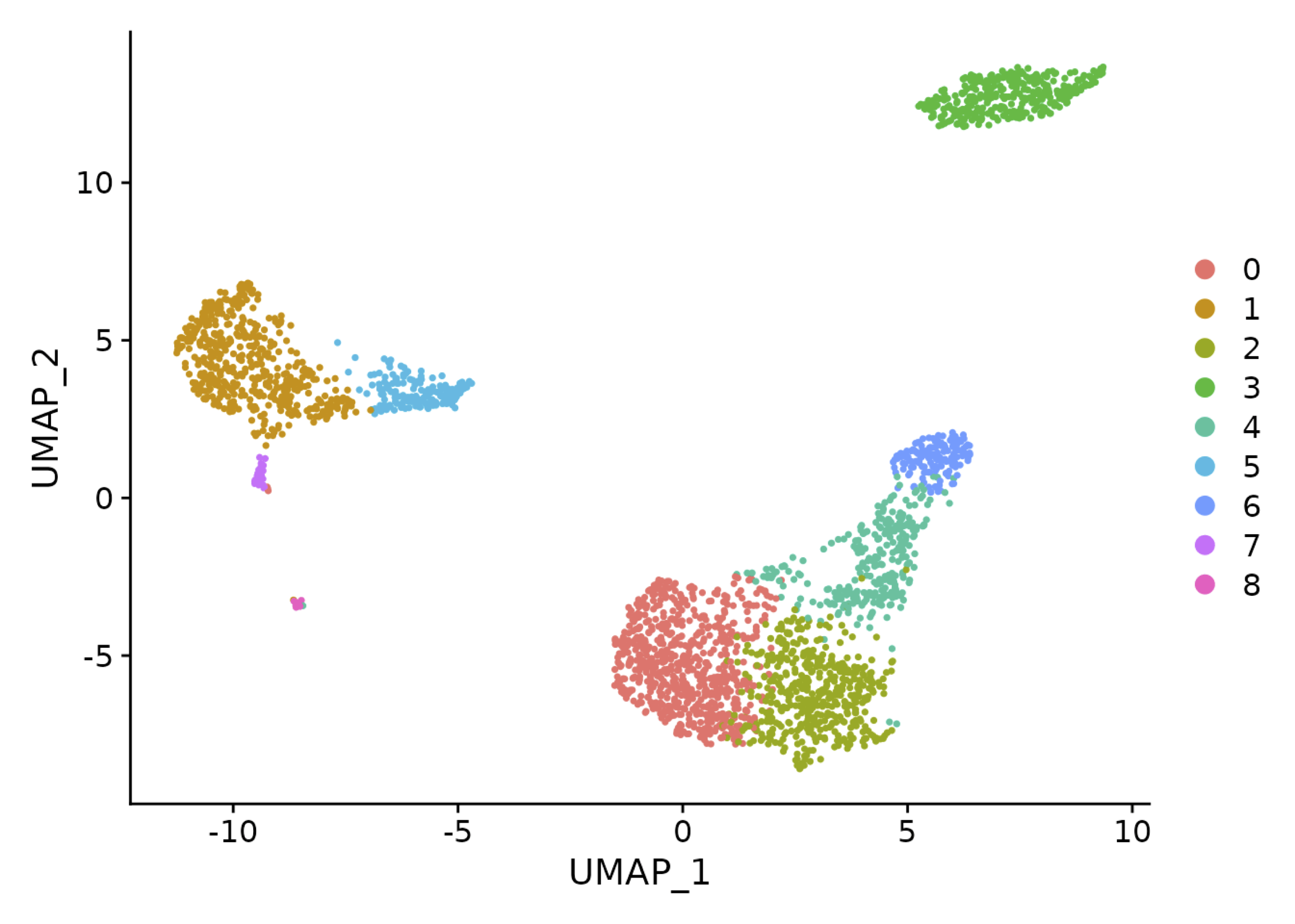
- Dimensionality Reduction: PCA, UMAP
- Clustering: cell type clusters
- Differential Gene Expression
Seurat
Most used tool
Good documentation
Several tutorials
Many methods
Extendable
Gene Expression Dynamics
Statistical Analysis of Differences Between Clusters
- Different types of hits
- Quantitatively significant between clusters
- Qualitatively different (predictive) of cluster membership
- Different types of markers
- Global: Distinguish one cluster from all of the others
- Local: Distinguish one cluster from a set of clusters
Comparing Gene Expression Across Groups
- Suppose you have two groups of cells
- You have expression levels for each cell within each group
- Question: is gene expression significantly different between both groups?
Methods
- Non-parametric: Wilcoxon rank sum test
- Parametric: t-test, negative binomial
- Classification: ROC
- Specialized: MAST
FindMarkers(data, ident.1 = "g1", ident.2 = "g2",
            group.by = "status", test.use = "roc",
            only.pos = TRUE)
Wilcoxon rank sum test
- Challenge: scRNA-seq data does not follow a beautiful bell-shaped curve
- Non-parametric: doesn’t make assumption about the shape of the data
- Rank-based: doesn’t use the magnitude of the expression levels but relies on the order of the data instead
- Two-sample: compares two independent groups
Wilcoxon rank sum test: step-by-step
- Combine: pool the expression levels from both groups
- Rank: sort the values from smaller to largest, assigning ranks (1, 2, …)
- Sum: sum the ranks for each group
- Test: the test determines if the difference in rank sums is large enough to be unlikely due to chance alone (p-value)
t-test
- Works better when data follow a bell-shaped distribution
- But has very good performance even when the data is not normally distributed
- Compares the average gene expression in the two groups
- Assesses if the difference is likely due to chance or a real effect of the groups
t-test: step-by-step
- Calculate the Means: Find the average gene expression for each group.
- Measure the Spread: How much the individual measurements vary around the averages (SD).
- Calculate the t-statistic: A number that combines the difference in means and the spread. Larger t-values suggest a bigger difference between groups.
- Get the p-value: The probability of seeing a difference as large as (or larger than) the one you observed if there was actually no real effect of the groups.
Negative Binomial Test
- Compares the expression between groups using count data
- In scRNA-seq, we count how many times each gene is expressed in a cell
- Count data doesn’t behave like other types of data (e.g., heights, weights). It has unique properties:
- Discrete: You can’t see a gene 0.5 times. Counts are whole numbers (0, 1, 2, etc.).
- Overdispersed: The variation in counts is often larger than expected from a simple model. Think of it as some genes being much more expressed than others.
Negative Binomial Distribuition
The negative binomial distribution is a statistical model that’s well-suited for count data. It can handle:
- Discrete nature: It only deals with whole numbers.
- Overdispersion: It allows for extra variation in the data.
- Overdispersion in scRNA-seq data means technical variability (technical features, like library preparation, sequencing) combined with biological variability (variability across cells).
The Negative Binomial Test: Comparing Groups
In scRNA-seq, we often want to compare gene expression between groups (e.g., treated vs. control cells). The negative binomial test helps us do this by:
- Modeling the Counts: It estimates the parameters of the negative binomial distribution for each group.
- Testing for Differences: It assesses whether the differences in counts between groups are statistically significant.
- p-values are often used to summarize evidences of differences between groups.
Simulation
- 33k genes
- 200 cells per group
- 2 groups
- 1k differentially expressed genes
- baseline counts: 10
- effect size: 5
DE Genes
| Correction | Wilcoxon | t-test | Negative Binomial | MAST |
|---|---|---|---|---|
| p-value | 0.91 | 0.97 | 0.97 | 0.09 |
| FDR | 0.49 | 0.72 | 0.76 | 0.00 |
Remember: we simulated data, so we know that there are 1.000 genes that are differentially expressed. The proportions above represent how much of these 1.000 genes each method was able to detect.
not DE Genes
| Correction | Wilcoxon | t-test | Negative Binomial | MAST |
|---|---|---|---|---|
| p-value | 0.05 | 0.05 | 0.05 | 0.02 |
| FDR | 0.00 | 0.00 | 0.00 | 0.00 |
Remember: we simulated data, so we know that there are 32.000 genes that are not differentially expressed. The proportions above represent how much of these 32.000 genes each method was able to detect as being differentially expressed (therefore, the method made mistakes).
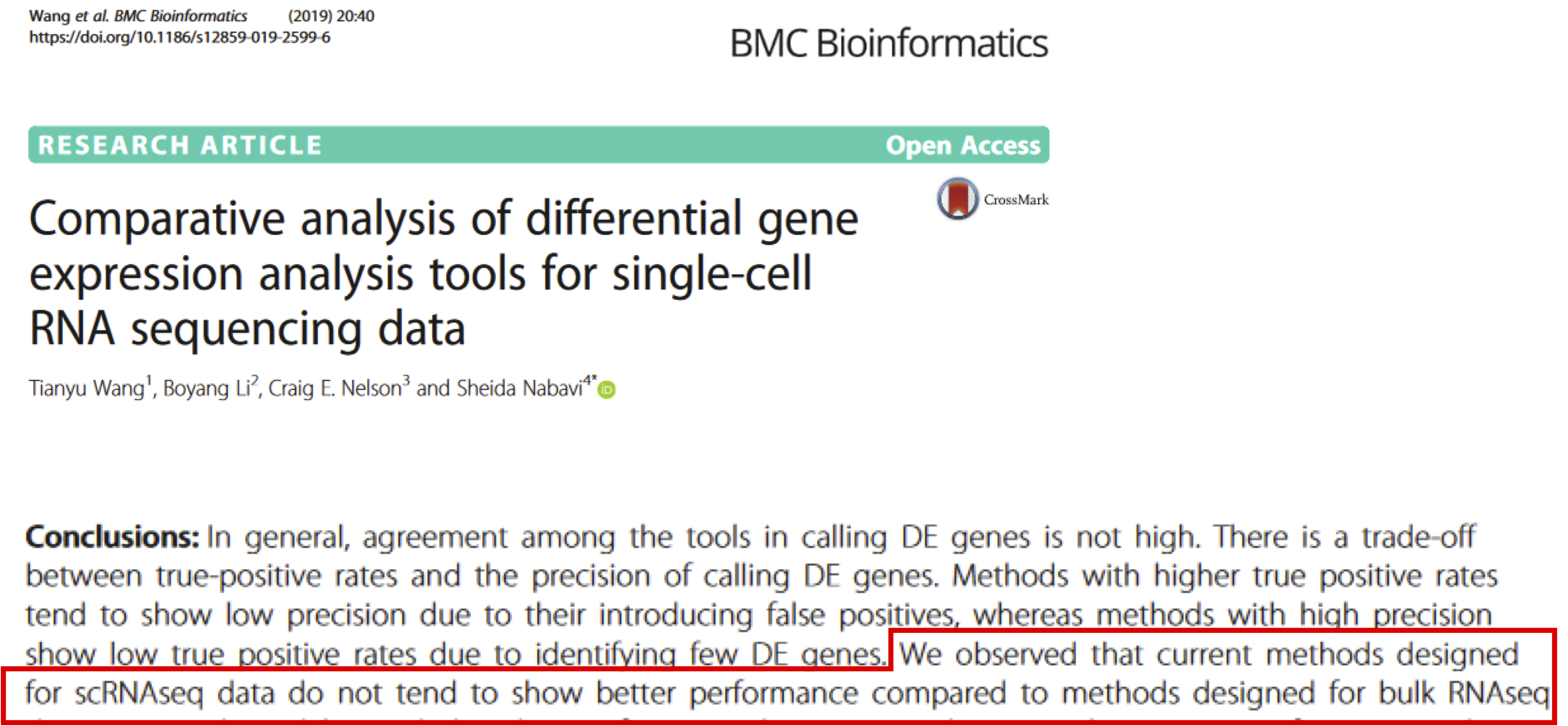
What about new methods?
Cell Type Annotation
Why annotate cell types?
- Interpreting the findings of our analysis is the most difficult task in sc-data analysis
- Understanding the biological state of each cluster is way harder then assigning clusters
- To do this, we need to “connect” our dataset to existing knowledge
- One strategy is to compare the expression of our dataset to the expressions of curated existing datasets (references)
- What tool do we use? SingleR
Cell Type Annotation
- SingleR pkg contains the statistical method for assignment
- celldex pkg shares several reference (well curated) datasets
- Most references are built from bulk RNA-seq and microarray
- They are good enough for annotation of sc-data, provided that the references contains the cell types that are expected to be present on the test data
- We’ll use a reference built from Blueprint and ENCODE data
- Single-cell references can also be used
How to perform annotation?
## Load the references
library(celldex)
ref = BlueprintEncodeData()

## We could load a sc reference instead
## ref = MuraroPancreasData()
How to perform annotation?
## Compare expression levels from my.data
##     to the reference
library(SingleR)
pred = SingleR(test = my.data, ref = ref,
               labels = ref$label.main)

table(pred$labels)
Observing the results
plotScoreHeatmap(pred)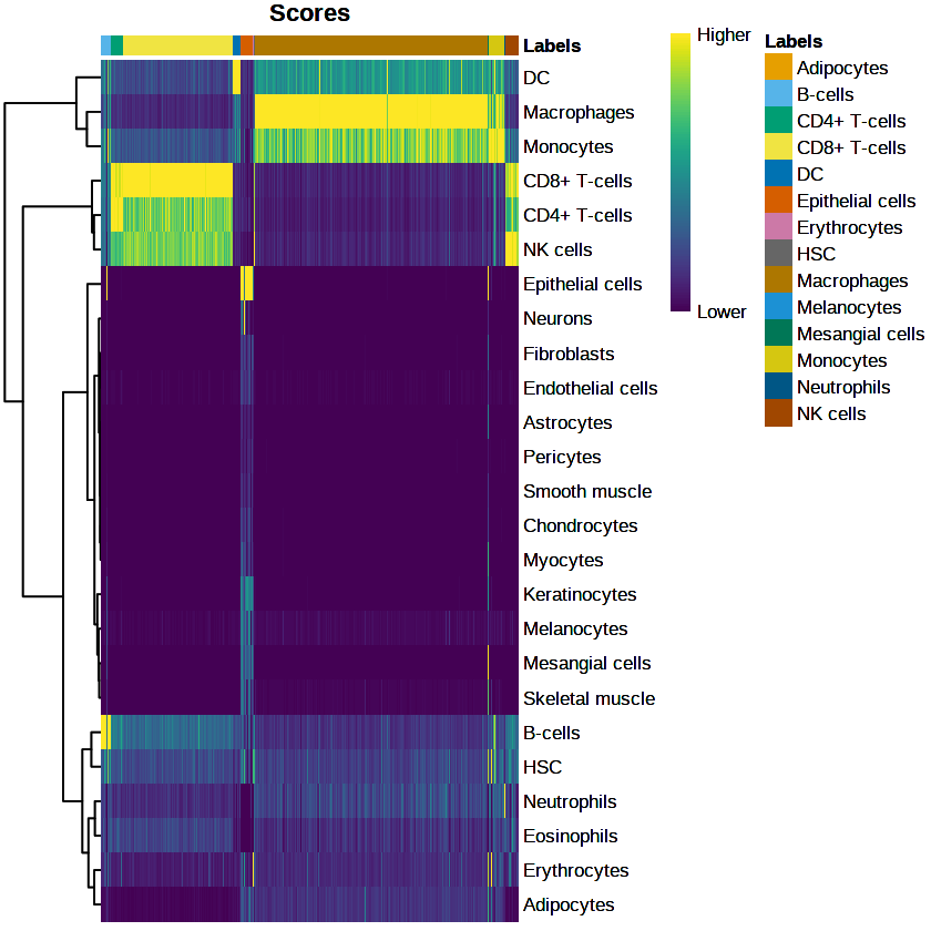

Differential Expression and Annotation